Bicycle Model

Simple Kinematic

Most simple one. Used for planning in the literature. See Motion Planning and Control Pipeline for a Formula Student Autonomous Vehicle, page 23

This model is well known in the literature (e.g. [14]) to perform well at low speed profiles (less than 5 m/s) Motion Planning and Control Pipeline for a Formula Student Autonomous Vehicle, page 23

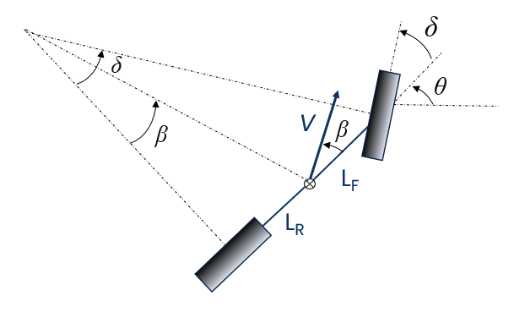
Here we use $\psi$ instead of $\theta$.

State space

$$X=\left[\begin{array}{c}x\\ y\\ \psi \\ v\end{array}\right]$$

and the state derivative is

$$\dot{X}=\left[\begin{array}{c}\dot{x}\\ \dot{y}\\ \dot{\psi }\\ \dot{v}\end{array}\right]=\left[\begin{array}{c}v\cos (\psi +\beta )\\ v\sin (\psi +\beta )\\ v\tan \delta \cos \beta /L\\ a\end{array}\right]$$

where

$$\beta =\arctan \left(\frac{L_r}{L_r+L_f}\tan \delta \right)$$

and the control inputs are

$$U=\left[\begin{array}{c}a\\ \delta \end{array}\right]$$

AMZ

Kinematic

This is model to be used in blending.

$$X=\left[\begin{array}{c}x\\ y\\ \psi \\ v_x\\ v_y\\ \omega \end{array}\right]\text{ , }U=\left[\begin{array}{c}a\\ \delta \end{array}\right]$$

and

$$\dot{X}=f(X,U,\dot{U})=\left[\begin{array}{c}{v}_x\cos \psi -v_y\sin \psi \\ x_x\sin \psi +v_y\cos \psi \\ \omega \\ \frac{F_x}{m}\\ \frac{L_r}{L_r+L_f}(\dot{\delta }{v}_x+\delta \dot{v_x})\\ \frac{1}{L_r+L_f}(\dot{\delta }{v}_x+\delta \dot{v_x})\end{array}\right]$$

Dynamic

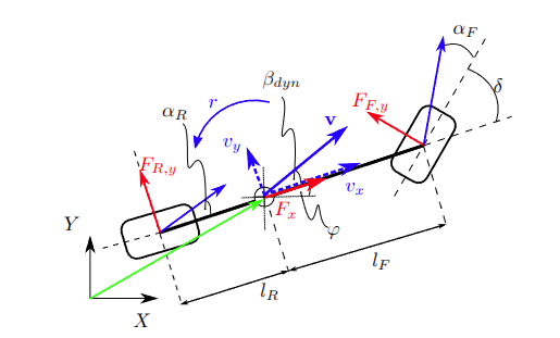
The used vehicle model is derived under the following assumptions,

• the vehicle drives on a flat surface
• load transfer can be neglected
• combined slip can be neglected
• the longitudinal drive-train forces act on the center of gravity. AMZ Driverless, The Full Autonomous Racing System, page 26

$$X=\left[\begin{array}{c}x\\ y\\ \psi \\ v_x\\ v_y\\ \omega \end{array}\right]\text{ , }U=\left[\begin{array}{c}a\\ \delta \end{array}\right]$$

and

$$\dot{X}=f(X,U)=\left[\begin{array}{c}{v}_x\cos \psi -v_y\sin \psi \\ x_x\sin \psi +v_y\cos \psi \\ \omega \\ \frac{1}{m}(F_{r,x}-F_{f,y}\sin \delta +m{v}_y\omega )\\ \frac{1}{m}(F_{r,y}+F_{f,y}\cos \delta -m{v}_x\omega )\\ \frac{1}{I_z}(F_{f,y}\cos \delta L_f-F_{r,y}{L}_r)\end{array}\right]$$

where we find lateral tire force by using simplified Pajecka tire model:

$$\begin{array}{rl}{\alpha }_r& =\arctan \left(\frac{v_y-L_r\omega }{v_x}\right)\\ F_{r,y}& =D_r\sin (C_r\arctan (B_r{\alpha }_r))\end{array}$$

and

$$\begin{array}{rl}{\alpha }_f& =\arctan \left(\frac{v_y+L_f\omega }{v_x}\right)-\delta \\ F_{f,y}& =D_f\sin (C_f\arctan (B_f{\alpha }_f))\end{array}$$

Where $F_X=f_M(P)-C_r-\frac{1}{2}{\rho }_{air}A{C}_d{v}_x^2$. Here $f_M(P)$ stands for motor force where $f_M$ is motor model and $P\in [-1,1]$ is the pedal position. These parameters are identified from the experiments.

Hybrid-Bicycle Model

This model blends the kinematic model and dynamic model based on the vehicle longitudinal speed.

Here observe that both models use the same state vector. Therefore we blend these model dynamics by

$$\dot{X}=f(X,U,\dot{U})=\lambda f_{dyn}(X,U)+(1-\lambda )f_{kin}(X,U,\dot{U})$$

where $\lambda =min\left(max\left(\frac{v_x-3}{5-3},0\right),1\right)$ when model is blended between $(3,5)$ m/s.

Discretization

We use 4th order Runge-Kutta method to discretize the the system.

Numerically Stable Dynamic Bicycle

$$X=\left[\begin{array}{c}x\\ y\\ \psi \\ v_x\\ v_y\\ \omega \end{array}\right]\text{ , }U=\left[\begin{array}{c}a\\ \delta \end{array}\right]$$

and we discretize that model using something similar to Backwards Euler method. See Numerically Stable Dynamic Bicycle Model for Discrete-time Control, page 2

$$X_{k+1}=\left[\begin{array}{c}{x}_{k+1}\\ y_{k+1}\\ {\psi }_{k+1}\\ v_{x,k+1}\\ v_{y,k+1}\\ {\omega }_{k+1}\end{array}\right]=\left[\begin{array}{c}{x}_k+\Delta t(v_{x,k}\cos {\psi }_k-v_{y,k}\sin {\psi }_k)\\ y_k+\Delta t(v_{y,k}\cos {\psi }_k+v_{x,k},\sin {\psi }_k)\\ {\psi }_k+\Delta t{\omega }_k\\ v_{x,k}+\Delta t{a}_k\\ \frac{m{v}_{x,k}+\Delta t\left[{\omega }_k(L_f{k}_f-L_r{k}_r)-k_f{\delta }_k{v}_{x,k}-m{v}_{x,k}^2{\omega }_k\right]}{m{v}_{x,k}-\Delta t(k_f+k_r)}\\ \frac{I_z{v}_{x,k}{\omega }_k+\Delta t\left[v_{y,k}(L_f{k}_f-L_r{k}_r)-L_f{k}_f{\delta }_k{v}_{x,k}\right]}{I_z{v}_{x,k}-\Delta t(L_f^2{k}_f+L_r^2{k}_r)}\end{array}\right]$$